Comparison sorting and the n log n bound

Sorting is the canonical algorithmic problem: the workhorse for search, statistics, and most data processing. Merge sort and quicksort both achieve $O(n \log n)$ time by splitting and recombining, but with different tradeoffs in memory and worst-case behavior[1]. A short information-theoretic argument shows that $n \log n$ is the floor for any comparison-based sort[2, 3].

Merge sort

Merge sort is divide-and-conquer:

1. Split the array in half.
2. Recursively sort each half.
3. Merge the two sorted halves into one sorted array.

The merge step walks two sorted arrays with a pointer in each, copying the smaller front element into the output until both are exhausted. This is $O(n)$ for arrays of total length $n$.

The recursion has depth $\log_2 n$ and does $O(n)$ work at each level (every element participates in exactly one merge at each level), giving total work $O(n \log n)$. Merge sort is stable (equal elements keep their relative order) and has a worst-case $O(n \log n)$ guarantee, but it needs $O(n)$ auxiliary space.

Quicksort

Quicksort is also divide-and-conquer, but it splits by value rather than by position:

1. Pick a pivot element.
2. Partition the array into elements $<$ pivot, elements $=$ pivot, and elements $>$ pivot.
3. Recursively sort the two outer partitions.

Partitioning can be done in place in $O(n)$ time using two pointers. The merging step is trivial: the partitions are already in the right relative order.

Average vs worst case. If the pivot splits the array roughly in half each time, the recursion is $\log_2 n$ deep with $O(n)$ work per level: $O(n \log n)$ total. If the pivot is always the minimum or maximum (worst case, achieved on a sorted array with a poor pivot rule), the recursion is $n$ deep with $O(n)$ work per level: $O(n^2)$. Randomizing the pivot choice makes the expected behavior $O(n \log n)$ regardless of input. Production implementations use median-of-three or other robust pivots and fall back to heapsort if recursion gets too deep (introsort).

Quicksort is in-place ($O(\log n)$ stack space) and typically faster in practice than merge sort because of better cache locality, at the price of the worst-case quadratic risk.

The $n \log n$ lower bound

Any comparison-based sort can be modeled as a decision tree: every internal node asks "is $a_i < a_j$?" and branches on the answer; every leaf labels a permutation of the input. For the algorithm to correctly sort every possible input, the tree must have at least $n!$ leaves, one per possible permutation.

A binary tree with $L$ leaves has height at least $\log_2 L$. So any comparison-based sort, in the worst case, performs at least

comparisons (using Stirling's approximation $\log_2(n!) = n \log_2 n - n \log_2 e + O(\log n)$). Merge sort and heapsort achieve this bound; quicksort matches it on average. No algorithm that only compares pairs of elements can do better.

(Sorts that look at the bits of the values, like counting sort and radix sort, can beat $n \log n$ at the cost of restrictions on the input domain.)

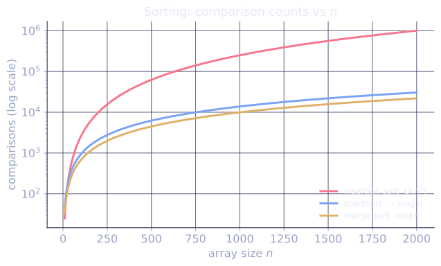
Check it on arrays

import random

def merge_sort(a):
    if len(a) <= 1: return a
    m = len(a) // 2
    L, R = merge_sort(a[:m]), merge_sort(a[m:])
    out, i, j = [], 0, 0
    while i < len(L) and j < len(R):
        if L[i] <= R[j]: out.append(L[i]); i += 1
        else:            out.append(R[j]); j += 1
    out.extend(L[i:]); out.extend(R[j:])
    return out

def quicksort(a):
    if len(a) <= 1: return a
    pivot = a[random.randrange(len(a))]              # randomized pivot
    less    = [x for x in a if x < pivot]
    equal   = [x for x in a if x == pivot]
    greater = [x for x in a if x > pivot]
    return quicksort(less) + equal + quicksort(greater)

rng = random.Random(0)
data = [rng.randint(0, 1000) for _ in range(500)]
random.seed(1)
print("merge sort matches sorted():", merge_sort(data) == sorted(data))
print("quicksort  matches sorted():", quicksort(data) == sorted(data))

# Stability test: equal keys keep original order in merge sort
pairs = [(1, 'a'), (2, 'b'), (1, 'c'), (2, 'd')]
stable = merge_sort(pairs)
print("merge sort is stable:", stable == [(1, 'a'), (1, 'c'), (2, 'b'), (2, 'd')])

# Worst-case quicksort with a deterministic-bad pivot (first element) on sorted input
# would be O(n^2); randomized pivot avoids it.
import math
print(f"log2(n!) for n=500 ~ {math.lgamma(501)/math.log(2):.0f} comparisons (n log n lower bound)")

Both algorithms reproduce the library sort, merge sort preserves the relative order of equal keys, and the decision-tree bound predicts the $n \log n$ comparison count.

Exercises

Exercise 1. Trace the merge step on the two sorted halves $[1, 4, 7]$ and $[2, 3, 8]$. Show the output after each comparison, and count the comparisons performed.

Exercise 2. The comparison lower bound uses $\log_2(n!) = \Theta(n \log n)$. Prove the upper half of that bound, $\log_2(n!) \le n \log_2 n$, directly from the definition of $n!$.

Exercise 3 (code). Counting sort beats the $n \log n$ bound on integers in a small range by reading values instead of comparing them. Implement it for nonnegative integers in $[0, K)$ in $O(n + K)$ time, and assert it matches the library sort on random data.

import random

def counting_sort(a, K):
    counts = [0] * K
    for x in a:               # tally each value: O(n)
        counts[x] += 1
    out = []
    for v in range(K):        # emit values in order: O(K + n)
        out.extend([v] * counts[v])
    return out

rng = random.Random(0)
K = 100
data = [rng.randrange(K) for _ in range(2000)]
assert counting_sort(data, K) == sorted(data)
print("counting sort matches sorted()")

The next lesson abstracts the divide-and-conquer pattern itself and the master theorem for its recurrences.

References

- [1]Cormen, T. H., Leiserson, C. E., Rivest, R. L., & Stein, C. (2009). Introduction to Algorithms (3rd ed.). MIT Press. Merge sort, quicksort, and their analysis (Ch. 2, 7).↩
- [2]Cormen, T. H., Leiserson, C. E., Rivest, R. L., & Stein, C. (2009). Introduction to Algorithms (3rd ed.). MIT Press. The decision-tree lower bound for comparison sorts (§8.1).↩
- [3]Knuth, D. E. (1998). The Art of Computer Programming, Vol. 3: Sorting and Searching (2nd ed.). Addison-Wesley. The definitive treatment of sorting and the comparison lower bound (§5.3).↩