Asymptotic complexity and Big-O

When the input doubles, does the running time double, square, or stay the same? Asymptotic complexity answers this with a precise notation that ignores constants and low-order terms, the only ones that matter once inputs are large[1]. Amortized analysis extends the same idea to operations whose individual costs vary but whose average over a long sequence is what counts[2].

Big-O notation

$T(n) = O(f(n))$ if there exist constants $c, n_0 > 0$ such that

Big-O is an upper bound that hides constants and low-order terms. Saying $T(n) = O(n^2)$ means the running time grows no faster than quadratically, eventually. A program with $T(n) = 100 n^2 + 50 n + 7$ is $O(n^2)$; so is one with $T(n) = n^2$.

The hidden constants matter in practice but not for distinguishing algorithms whose growth rates differ. An $O(n \log n)$ algorithm with a large constant beats an $O(n^2)$ one for large enough $n$, regardless of how large the constants are.

Big-Omega and Big-Theta

Big-Omega is the matching lower bound: $T(n) = \Omega(f(n))$ if there exist $c, n_0$ with $T(n) \ge c\,f(n)$ for $n \ge n_0$. Big-Theta is both at once, $T(n) = \Theta(f(n))$ when $T(n) = O(f(n))$ and $T(n) = \Omega(f(n))$: a tight characterization, the actual growth rate.

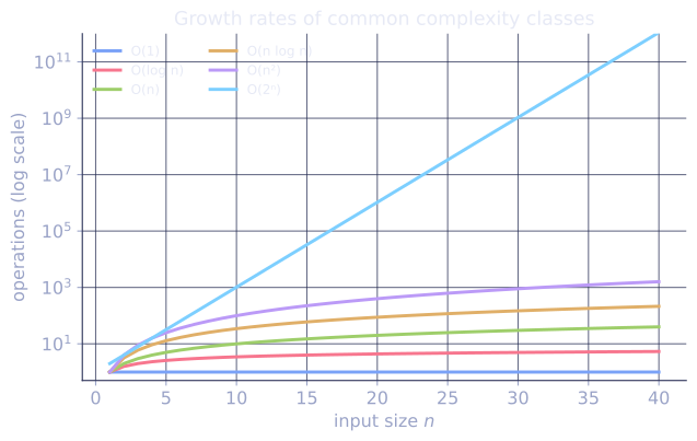
The hierarchy of common complexity classes:

Each class is strictly smaller (so an $O(n)$ algorithm is also $O(n^2)$ but not the reverse). The exponential jumps are the practical cliffs: $n = 100$ takes microseconds at $O(n^2)$, milliseconds at $O(n^3)$, and longer than the age of the universe at $O(n!)$.

Worst, average, and best case

Big-O usually refers to the worst case: the maximum running time over all inputs of size $n$. Average case averages over an input distribution, often uniform. Best case is the minimum. Quicksort is $O(n^2)$ worst case, $O(n \log n)$ average case; binary search is $O(\log n)$ worst, $O(1)$ best (key at the middle). Worst-case bounds are the safe default for guarantees; average-case bounds reflect typical behavior under stated input assumptions.

Amortized analysis

Some operations are usually cheap but occasionally expensive. The right cost is the amortized cost: total cost of a sequence of $n$ operations divided by $n$.

The canonical example is a dynamic array that doubles its capacity when it fills up. Most append calls are $O(1)$, but every $k$-th call (when full) is $O(k)$ because all elements must be copied to a new larger buffer. Across $n$ inserts, the expensive ones at sizes $1, 2, 4, \dots, n/2, n$ cost $1 + 2 + 4 + \cdots + n \le 2n$ total. The cheap ones contribute $n$ more. The total is $\le 3n$, so the amortized cost per insert is $O(1)$, even though individual inserts can be $O(n)$.

Check it on arrays

import time, random, sys
sys.setrecursionlimit(10_000)

# Empirical growth rates: time three algorithms over increasing n.
def linear_sum(n):
    s = 0
    for x in range(n):
        s += x
    return s

def quadratic_pairs(n):
    s = 0
    for i in range(n):
        for j in range(n):
            s += 1
    return s

def n_log_n(n):                                      # merge-sort style work
    if n <= 1: return 0
    return n + n_log_n(n // 2) + n_log_n(n - n // 2)

def timeit(f, n):
    t = time.perf_counter()
    f(n)
    return time.perf_counter() - t

# Growth-rate fingerprint: t(2n)/t(n) approaches 2 for O(n), 4 for O(n^2), ~2.2 for n log n
sizes = [200, 400, 800, 1600]
print("size  | linear    quad      n log n")
for n in sizes:
    print(f"{n:>5} | {timeit(linear_sum, n):.5f}  {timeit(quadratic_pairs, n):.5f}  {timeit(n_log_n, n):.5f}")

# Amortized O(1) append: total work for n appends is < 3n, not n^2
class DynArray:
    def __init__(self): self.cap = 1; self.size = 0; self.data = [None]
    def append(self, x):
        if self.size == self.cap:                    # double on full
            new = [None] * (self.cap * 2)
            for i in range(self.size): new[i] = self.data[i]
            self.data = new; self.cap *= 2
        self.data[self.size] = x; self.size += 1

n = 100_000
arr = DynArray()
t = time.perf_counter()
for i in range(n): arr.append(i)
elapsed = time.perf_counter() - t
print(f"{n} appends: {elapsed:.4f}s  per-op {elapsed/n*1e6:.2f} us")

The doubling fingerprint matches the predicted growth (around 2, 4, and a bit over 2), and 100,000 dynamic-array appends complete in linear time despite individual expensive resizes.

Exercises

Exercise 1. Prove directly from the definition that $T(n) = 3n^2 + 10n + 7$ is $O(n^2)$. Give explicit constants $c$ and $n_0$.

Exercise 2. Show that $O(n)$ is a strict subset of $O(n^2)$: prove every function in $O(n)$ is in $O(n^2)$, then exhibit one function in $O(n^2)$ that is not in $O(n)$.

Exercise 3 (code). The lesson claims doubling makes $n$ appends cost $\le 3n$ total. Instrument a doubling dynamic array to count the total number of element copies (work done during resizes) across $n = 100000$ appends, and assert the count is below $2n$ (the geometric-series bound on copy work).

import numpy as np

def total_copies(n):
    cap, size, copies = 1, 0, 0
    for _ in range(n):
        if size == cap:            # resize: copy all current elements
            copies += size
            cap *= 2
        size += 1
    return copies

n = 100_000
c = total_copies(n)
# Copies are 1+2+4+...+the last power of two below n, a geometric sum < 2n.
assert c < 2 * n
print("total copies:", c, "  bound 2n =", 2 * n)

The next lesson formalizes this dynamic array and the hash map.

References

- [1]Cormen, T. H., Leiserson, C. E., Rivest, R. L., & Stein, C. (2009). Introduction to Algorithms (3rd ed.). MIT Press. Asymptotic notation and growth of functions (Ch. 3).↩
- [2]Cormen, T. H., Leiserson, C. E., Rivest, R. L., & Stein, C. (2009). Introduction to Algorithms (3rd ed.). MIT Press. Amortized analysis, including the aggregate and potential methods (Ch. 17).↩