Test-time compute scaling

The scaling laws for pretraining tell us that spending more compute during training improves model quality. A complementary axis: spending more compute at inference time.

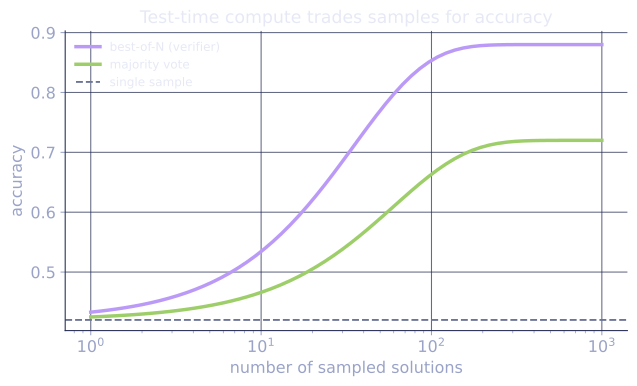
Test-time compute scaling (Snell et al., 2024; Lightman et al., 2023) shows that with the right search algorithms and verifiers, allocating more inference FLOPs can match the gains from training a much larger model[1].

Why test-time compute helps

An LLM generates one token at a time, conditioned on previous tokens. Each token is one inference step. A 100-step chain of thought uses 100x more inference compute than a one-token answer -- and as CoT demonstrated, this extra compute improves accuracy.

Test-time compute scaling extends this: instead of one linear chain of thought, search over a tree of reasoning paths[2]. More compute = explore more branches = higher probability of finding the correct answer.

Process reward models (PRMs)

To guide search, we need a verifier that evaluates intermediate reasoning steps, not just the final answer. An outcome reward model (ORM) scores only the final answer; a process reward model (PRM) scores each step.

Training a PRM:

• Collect human annotations on the correctness of individual reasoning steps.
• Or use process supervision with Monte Carlo rollouts: given a partial solution up to step $k$, estimate the probability of reaching the correct answer by sampling $N$ random continuations and checking which succeed.

PRM scores $r_k \in [0, 1]$ for each step $k$ indicate whether the step is correct. The minimum score along a path gives the path quality.

Search algorithms with PRMs

Best-of-N sampling

Generate $N$ complete solutions independently, score each with an ORM or PRM, and return the best:

$$y^* = \arg\max_{y_1, \dots, y_N} r_{\text{ORM}}(x, y_i).$$

Simple but requires generating $N$ full solutions. Effective when $N$ is large.

Beam search with process rewards

Use the PRM to prune a beam during step-by-step generation:

1. Start with beam width $B$ at step 0.
2. At each step, expand all current beams by sampling $k$ continuations each.
3. Score each candidate continuation with the PRM.
4. Keep the top-$B$ candidates (pruning the rest).
5. Continue until all beams are complete.

This focuses computation on the most promising reasoning paths.

Monte Carlo Tree Search (MCTS)

Model search as a tree:

• Nodes: partial reasoning traces.
• Edges: possible next steps.
• Value function: PRM score at leaf; Monte Carlo rollouts for non-leaves.

MCTS uses UCB (Upper Confidence Bound) to balance exploration (trying new branches) and exploitation (continuing promising branches):

$$\text{UCB}(n) = V(n) + c \sqrt{\frac{\ln N_{\text{parent}}}{N(n)}},$$

where $V(n)$ is the estimated value, $N(n)$ the visit count, and $c$ controls exploration.

OpenAI o1 and o3

OpenAI's o1 and o3 models ("reasoning models") are trained with RLHF on long chains of thought and apply test-time compute scaling. Key characteristics:

• Long reasoning traces: models generate 1,000-100,000 reasoning tokens before answering.
• Hidden reasoning: the reasoning chain ("thinking" tokens) is not shown to the user (only the final answer is).
• Token budget: the API allows controlling how many "reasoning tokens" to allocate. More tokens = more compute = better answers.
• Training: GRPO or PPO with outcome-based verification rewards on math and code problems.

Scaling curve: o1-preview significantly outperforms GPT-4o on AIME (math competition) at 25x more inference compute; o3 at 100x compute budget approaches human expert level.

DeepSeek-R1

DeepSeek-R1 (DeepSeek, 2025) achieves comparable reasoning to o1 using GRPO with verifiable math and code rewards. Key insights:

• Cold start with a small amount of long-CoT SFT data (before GRPO) prevents early reward hacking and stabilizes training.
• Multi-stage pipeline: base model → SFT on long-CoT → GRPO with math/code rewards → rejection sampling (keep top-k GRPO outputs) → SFT on filtered data → GRPO again.
• Emergent self-reflection: the model learns to check its own answers, backtrack on errors, and try multiple approaches -- without explicit supervision of these behaviors.
• Distillation: smaller models (1.5B-14B) trained to imitate R1's reasoning traces achieve strong performance without the full RL training.

Compute allocation tradeoffs

Approach	Training compute	Inference compute	Best for
Larger pretrained model	High	Low (per token)	Broad capability
Best-of-N sampling	Low	Medium	Any verifiable task
PRM + beam search	Medium (PRM training)	Medium	Step-by-step math
MCTS	Low	High	Complex reasoning
o1-style (GRPO + long CoT)	Medium (RL)	Very high	Math, code, science

Exercises

Exercise 1. A model solves a problem correctly with probability $0.4$ per independent attempt, and a perfect verifier can always identify a correct solution when one is present. Under best-of-N (return any correct attempt the verifier finds), compute the success probability for $N = 1, 4, 16$. Why does this argument require a verifier, and how would the picture change if instead you used a majority vote?

Solution

Step 1. Best-of-N with a perfect verifier succeeds if at least one of the $N$ attempts is correct. The failure probability is $(1 - 0.4)^N = 0.6^N$, so $P(\text{success}) = 1 - 0.6^N$.

Step 2. Evaluate:

$$N = 1: 1 - 0.6 = 0.40, \quad N = 4: 1 - 0.6^4 = 1 - 0.1296 = 0.8704, \quad N = 16: 1 - 0.6^{16} \approx 0.9997.$$

Step 3. The verifier is what lets a single correct attempt win even when it is the minority, so accuracy climbs toward 1 as $N$ grows. Majority vote has no such guarantee: with per-attempt accuracy $0.4 < 0.5$, the wrong answers form the majority, so voting drives accuracy down as $N$ grows. Best-of-N needs a verifier precisely because it must recognize a rare correct answer rather than count votes.

Exercise 2. A reasoning model is offered two ways to spend extra inference compute on a 200-token base solution: (a) best-of-16 sampling, generating 16 independent length-200 chains; (b) one single chain extended to 3200 tokens. Both spend the same token budget. Express each budget in forward passes and state what each approach buys, referencing why a verifier matters for (a).

Solution

Step 1. Token cost is roughly one forward pass per generated token. Best-of-16 over length-200 chains costs $16 \times 200 = 3200$ forward passes. The single extended chain costs $3200$ forward passes. The budgets match.

Step 2. Best-of-16 spends the budget on breadth: 16 independent attempts that a verifier or vote selects among, raising the chance that at least one lands correctly. It needs a verifier (or a reliable vote) to pick the winner, otherwise the extra samples are wasted.

Step 3. The single long chain spends the budget on depth: more reasoning steps within one trajectory, allocating more computation to a single line of thought. It needs no selector but cannot recover if that one trajectory commits an early error. The two approaches trade breadth against depth at equal cost, and the better choice depends on whether a verifier is available and whether errors are better escaped by resampling or by more deliberation.

Exercise 3. Using the compute-allocation table in this lesson, recommend an approach for each setting and justify it from the training-versus-inference compute split: (a) a math-competition assistant where a checker can verify final answers and latency is not critical; (b) a high-volume autocomplete feature serving millions of requests per day where per-token latency must stay low.

Solution

Step 1. Setting (a): a verifiable task that tolerates latency. Best-of-N sampling (or PRM-guided search) fits: low training compute, medium-to-high inference compute, and the available checker is what makes the extra samples pay off. Snell et al.'s compute-matched result says a small model with best-of-N can match a much larger trained model here, as long as the verifier exists.

Step 2. Setting (b): high volume, latency-sensitive, no per-request verifier budget. A larger pretrained model fits: high training compute paid once, but low inference compute per token. Spending inference compute on search at this volume would multiply latency and serving cost on every request, which the autocomplete budget cannot absorb.

Step 3. The split is the deciding axis: test-time scaling moves cost from a one-time training bill to a recurring per-query bill, which is worth it when queries are rare, verifiable, and quality-critical, and a poor trade when queries are cheap, frequent, and latency-bound.

Snell et al. (2024) show that compute-matched comparisons favor test-time scaling for math: a small model with best-of-N can match a large model trained with much more compute, as long as a verifier is available[1].

---

References

1. [1]Snell, C., Lee, J., Xu, K., & Kumar, A. (2024). "Scaling LLM test-time compute optimally can be more effective than scaling model parameters". arXiv:2408.03314. The compute-matched argument for best-of-N and search over verifiers.↩
2. [2]Yao, S., et al. (2023). "Tree of thoughts: deliberate problem solving with large language models". NeurIPS. arXiv:2305.10601. Searching over a tree of reasoning paths rather than one linear chain.↩