Word2vec: CBOW and skip-gram

N-gram models treat vocabulary items as discrete symbols -- "cat" and "kitten" are as unrelated as "cat" and "democracy." Word embeddings map each token to a continuous vector such that semantically and syntactically related words land nearby. This geometric structure is not hand-coded; it emerges from predicting which words appear in which contexts.

The distributional hypothesis

"A word is characterized by the company it keeps" (Firth, 1957).

Words that appear in similar contexts tend to have similar meanings. "Bank" and "river" often co-occur (river bank); "bank" and "finance" also co-occur (financial bank). An embedding that captures co-occurrence statistics will place both senses of "bank" near their respective neighbors.

Two model architectures

CBOW (Continuous Bag of Words): predict the center word from its context. Skip-gram: predict context words from the center word.

Both architectures come from the original word2vec work[1]. Skip-gram with negative sampling (SGNS)[2] is the workhorse and produces better representations for rare words; we derive it in full.

Skip-gram with negative sampling

The full softmax over a $V$-word vocabulary is expensive. Negative sampling replaces it with a binary classification task:

For each (center $w$, context $c$) pair from the corpus, maximize:

where $\mathbf{v}_w$ is the center embedding of $w$, $\mathbf{u}_c$ is the context embedding of $c$, and $P_n(w) \propto f(w)^{3/4}$ is the noise distribution (unigram frequencies raised to the 3/4 power, which smooths the distribution toward rare words)[2]. $K \approx 5{-}15$ negative samples per positive pair.

The sigmoid $\sigma(x) = 1/(1 + e^{-x})$ turns dot products into probabilities. Maximizing $\log \sigma(\mathbf{v}_w \cdot \mathbf{u}_c)$ pushes true context pairs to high dot product; maximizing $\log \sigma(-\mathbf{v}_w \cdot \mathbf{u}_{c_k})$ pushes negative pairs to low dot product.

Why analogies emerge

After training, the embedding space satisfies:

This is not hand-engineered. It emerges because "king" and "queen" share all contexts except those relating to gender, while "man" and "woman" differ in exactly those gender-related contexts. The difference $\mathbf{v}_{\text{king}} - \mathbf{v}_{\text{queen}}$ encodes the gender direction, and adding $\mathbf{v}_{\text{woman}}$ traverses it.

Implementation with numpy

import numpy as np
from collections import Counter

# Toy corpus
sentences = [
    ["the", "cat", "sat", "on", "the", "mat"],
    ["the", "dog", "sat", "on", "the", "floor"],
    ["cats", "and", "dogs", "are", "animals"],
    ["animals", "live", "on", "the", "floor", "and", "mat"],
]
vocab = list(set(w for s in sentences for w in s))
w2i = {w: i for i, w in enumerate(vocab)}
V = len(vocab)

# Hyperparameters
d = 10        # embedding dimension
window = 2    # context window size
K = 3         # negative samples
lr = 0.05
n_epochs = 200

# Unigram^(3/4) noise distribution
counts = Counter(w for s in sentences for w in s)
noise_weights = np.array([counts[w] ** 0.75 for w in vocab])
noise_weights /= noise_weights.sum()

# Embeddings: center (V) and context (U)
rng = np.random.default_rng(42)
V_emb = rng.normal(0, 0.1, (V, d))   # center embeddings
U_emb = rng.normal(0, 0.1, (V, d))   # context embeddings

def sigmoid(x):
    return 1.0 / (1.0 + np.exp(-np.clip(x, -10, 10)))

# Build (center, context) training pairs
pairs = []
for sent in sentences:
    for i, center in enumerate(sent):
        for j in range(max(0, i - window), min(len(sent), i + window + 1)):
            if j != i:
                pairs.append((w2i[center], w2i[sent[j]]))

for epoch in range(n_epochs):
    total_loss = 0.0
    for wi, ci in pairs:
        # Positive sample
        score_pos = V_emb[wi] @ U_emb[ci]
        prob_pos  = sigmoid(score_pos)
        grad_pos  = (1 - prob_pos)
        # Negative samples
        neg_ids = rng.choice(V, size=K, p=noise_weights)
        grad_v  = grad_pos * U_emb[ci].copy()
        grad_uc = grad_pos * V_emb[wi].copy()
        for ni in neg_ids:
            score_neg = V_emb[wi] @ U_emb[ni]
            prob_neg  = sigmoid(-score_neg)   # want to be 0
            grad_neg  = -(1 - prob_neg)
            grad_v   += grad_neg * U_emb[ni]
            U_emb[ni] += lr * grad_neg * V_emb[wi]
            total_loss -= np.log(prob_neg + 1e-9)
        V_emb[wi] += lr * grad_v
        U_emb[ci] += lr * grad_uc
        total_loss -= np.log(prob_pos + 1e-9)
    if (epoch + 1) % 50 == 0:
        print(f"Epoch {epoch + 1}: loss = {total_loss:.2f}")

# Nearest neighbors of "cat"
query = V_emb[w2i["cat"]]
sims  = V_emb @ query / (np.linalg.norm(V_emb, axis=1) * np.linalg.norm(query) + 1e-9)
top5  = sims.argsort()[-5:][::-1]
print("\nNearest to 'cat':", [vocab[i] for i in top5])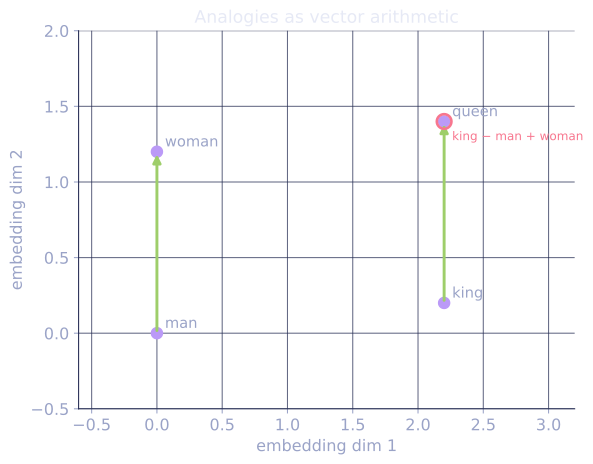

Exercises

Exercise 1. For a single positive (center, context) pair, the skip-gram objective is $\mathcal{L} = \log \sigma(\mathbf{v}_w \cdot \mathbf{u}_c)$. Derive $\partial \mathcal{L} / \partial \mathbf{v}_w$ by hand, then evaluate it for $\mathbf{v}_w = (0.5, -0.2, 0.3)$ and $\mathbf{u}_c = (0.1, 0.4, -0.1)$.

Exercise 2. The noise distribution is $P_n(w) \propto f(w)^{3/4}$. Take a two-word vocabulary with unigram frequencies $f(a) = 0.9$, $f(b) = 0.1$. Compute $P_n(a)$ and $P_n(b)$, and compare with the raw unigram probabilities. Which word does the $3/4$ power favor as a negative sample?

Exercise 3 (code). The skip-gram negative-sampling gradient is hand-derived in the implementation above. Verify the full gradient with respect to $\mathbf{v}_w$ (one positive context plus $K$ negatives) against a finite- difference estimate of the objective.

import numpy as np

def sigmoid(x):
    return 1.0 / (1.0 + np.exp(-x))

rng = np.random.default_rng(0)
d, K = 5, 4
v_w = rng.normal(0, 1, d)
u_c = rng.normal(0, 1, d)
U_neg = rng.normal(0, 1, (K, d))      # K negative context vectors

def objective(v):
    pos = np.log(sigmoid(v @ u_c))
    neg = np.sum(np.log(sigmoid(-(U_neg @ v))))
    return pos + neg

# Analytic gradient wrt v_w:
#   d/dv [log sigma(v.u_c)]      = (1 - sigma(v.u_c)) u_c
#   d/dv [log sigma(-v.u_k)]     = -(1 - sigma(-v.u_k)) u_k
g = (1 - sigmoid(v_w @ u_c)) * u_c
g -= np.sum((1 - sigmoid(-(U_neg @ v_w)))[:, None] * U_neg, axis=0)

# Central finite differences
eps = 1e-6
g_fd = np.zeros(d)
for i in range(d):
    e = np.zeros(d); e[i] = eps
    g_fd[i] = (objective(v_w + e) - objective(v_w - e)) / (2 * eps)

assert np.allclose(g, g_fd, atol=1e-5)
print("max abs diff:", np.abs(g - g_fd).max())

What word2vec captures (and misses)

Word2vec learns static embeddings: one vector per word type, regardless of context. "Bank" gets the same vector whether the sentence is about rivers or finance. This is the fundamental limitation that contextual embeddings (ELMo, BERT) address.

It also misses morphology: "play," "plays," "playing," and "played" are four separate vocabulary entries with independently trained embeddings. FastText (next lesson) fixes this by composing embeddings from character n-grams.