Gradient checkpointing

Training a deep network normally stores every intermediate activation during the forward pass, then reads them during backward to compute gradients. This memory grows linearly with depth and quickly becomes the limiting factor for large models. Gradient checkpointing drops most activations and recomputes them during the backward pass, trading extra compute for much less memory[1].

The memory problem

For a network with $L$ layers and activation size $A$ per layer, the backward pass needs all $L$ stored activations, costing $O(LA)$ memory.

For a 24-layer Transformer with 4096 hidden dim and batch 32 with sequence length 2048, activations alone consume tens of GB. Doubling the sequence length doubles activation memory; tripling batch size triples it.

This is often the bottleneck before parameter or gradient memory becomes the issue.

The basic idea

Conceptually:

1. Forward: compute and store only checkpoint activations (every $\sqrt{L}$ layers, say).
2. Backward: when you need a non-checkpointed activation, recompute it by running forward from the nearest earlier checkpoint.

This trades:

• Memory: $O(\sqrt{L}\, A)$ instead of $O(L A)$ for $L$ layers with $\sqrt{L}$ checkpoints.
• Compute: extra forward passes during backward, increasing training time by ~33%.

For most use cases, the memory savings are worth the time cost.

Why $\sqrt{L}$ checkpoints

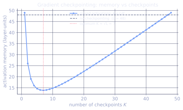
If you keep $K$ checkpoints, memory is $O(K + L/K)$ for the checkpoints plus the activations being recomputed for backward. The minimum is at $K \approx \sqrt{L}$, giving memory $O(\sqrt{L})$[1].

For a 100-layer network, this means keeping about 10 checkpoints and recomputing in 10-layer segments. Memory drops 10x; compute grows by the recomputation overhead.

In practice

Most frameworks have a built-in:

# PyTorch
from torch.utils.checkpoint import checkpoint

def transformer_block(x):
    return checkpoint(my_block, x)

The framework remembers which activations are needed, calls forward again at backward time, and stitches the resulting gradients into the overall backward pass.

Decisions:

• Which sublayers to checkpoint: typically per-Transformer-block, not per-individual-op. Per-block is the right granularity.
• Which layers to not checkpoint: usually the first and last layers, which the optimizer needs frequent access to.

Activation checkpointing in distributed training

Combined with data parallelism (DDP) and model parallelism (FSDP), gradient checkpointing is essential for training models too large to fit any other way.

For GPT-3-scale (175B parameters), checkpointing every Transformer block is non-negotiable: without it, activation memory exceeds any single GPU.

Selective recomputation

Modern recipes (selective gradient checkpointing) recompute only the expensive-to-store, cheap-to-recompute ops:

• LayerNorm, dropout, GELU: cheap to recompute, modest memory savings.
• Attention: expensive to recompute (quadratic), large memory savings.
• FFN: medium on both axes.

By picking the right ops, you can save more memory per FLOP than uniform checkpointing.

Megatron-LM and DeepSpeed support this with config switches.

Reversible architectures

A different memory trick: design the network so the forward pass is reversible (every layer has a closed-form inverse). Then activations don't need to be stored at all; they can be exactly reconstructed from the output during backward.

RevNet and Reformer apply this idea. Limited adoption because the architectural constraints (each block must be invertible) reduce flexibility.

When to use checkpointing

• Always when memory-limited: which is most large-model training.
• Skip when memory is abundant: small models fit comfortably; the extra compute is wasted.
• Skip when training is compute-limited: occasionally true on very fast hardware with abundant memory.

In practice, checkpointing is on by default in training pipelines for LLMs and large vision models.

The bigger context

Gradient checkpointing is one of several memory optimization techniques used in large-scale training:

• Activation recomputation (this lesson).
• Mixed precision (previous lesson).
• Optimizer state sharding (FSDP, ZeRO, next lessons).
• CPU offload: keep optimizer state in CPU memory, transfer to GPU for the update.
• Activation offload: similarly for activations.

Each saves memory at some compute cost. The combination is what makes billion-parameter and trillion-parameter training possible on real-world hardware.

Exercises

Exercise 1. A network has $L = 48$ transformer blocks. Each block, when stored, holds $A = 0.5$ GB of activations for the current batch. Compare the peak activation memory of full storage against $\sqrt{L}$ checkpointing, and state the speed cost.

Exercise 2. Derive that $K = \sqrt{L}$ minimizes the checkpoint memory. Treat memory as $M(K) = K + L/K$ (in units of one block's activations) and minimize over the number of checkpoints $K$.

Exercise 3. A team trains a 100-layer model. Plain training needs 80 GB of activation memory but only 60 GB fits on the GPU. They consider uniform $\sqrt{L}$ checkpointing (memory $\propto 2\sqrt{L}/L$ of full) versus selective checkpointing that recomputes only attention (cheap to recompute, half the activation footprint) and stores everything else. Estimate whether each option fits, and name the tradeoff that decides between them.

The next lesson covers the main scaling axis at the cluster level: data parallelism.

References

- [1]Chen, T., Xu, B., Zhang, C., & Guestrin, C. (2016). "Training deep nets with sublinear memory cost". arXiv:1604.06174. The source of the -memory checkpointing strategy.↩