Contrastive self-supervision

Labels are expensive; data is cheap. Contrastive self-supervised learning turns this asymmetry into representations: take an unlabeled image, make two augmented copies of it (a "positive pair"), and train the encoder to give them similar features while pushing apart features of different images. The InfoNCE loss formalizes this as a classification problem where each positive must beat many negatives.

The InfoNCE loss

van den Oord et al. (2018)[3]. Given an anchor representation $z$, its positive partner $z^+$, and $K$ negative partners $z^-_1, \dots, z^-_K$, the contrastive loss is

It is exactly the cross-entropy of identifying the positive in a $(K + 1)$-way classification. The temperature $\tau$ (typically 0.07-0.5) controls how sharply the model focuses on near-positives versus all negatives.

The loss minimizes a lower bound on the mutual information between the anchor and positive views (hence "InfoNCE" = "Noise Contrastive Estimation for Information").

SimCLR

Chen et al. (2020)[1].

Given a batch of $N$ images, apply two random augmentations to each, producing $2N$ views. Treat each view's other-augmented version as its positive; the other $2(N-1)$ views are negatives.

Architecture:

• Backbone $f$: a ResNet that produces a representation $h$.
• Projection head $g$: a small MLP that produces $z = g(h)$. The contrastive loss is computed in projection space.
• After pretraining, discard $g$ and use $h$ for downstream tasks.

Why a projection head? Empirically, putting the loss directly on $h$ hurt performance; an MLP gives the loss its own subspace and protects the representation from over-specialization.

Augmentations matter enormously. Standard ones for vision:

• Random resized crop.
• Random color jitter (brightness, contrast, saturation, hue).
• Gaussian blur.
• Random horizontal flip.

The composition is what generates "different views of the same scene". Stronger augmentations (more aggressive crops, more color jitter) give better representations.

SimCLR needs large batches (4096+) to provide enough negatives. This is its main practical limitation.

MoCo (Momentum Contrast)

He et al. (2020)[2]. Avoid SimCLR's huge-batch requirement by maintaining a queue of past representations as negatives.

Two encoders:

• Query encoder $f_q$: trained normally.
• Key encoder $f_k$: parameters are an exponential moving average of $f_q$'s.

For each batch:

1. Compute $z_q$ from the anchor view using $f_q$.
2. Compute $z_k$ from the positive view using $f_k$.
3. Pull from the queue of past $z_k$ values for many additional negatives.
4. Apply InfoNCE loss with $z_q$ as anchor, $z_k$ as positive, and the queue as negatives.
5. After the update, enqueue $z_k$ and dequeue the oldest entry.

Why the moving-average key encoder? Without it, recent queue entries come from a stale version of the network, hurting consistency. The slowly-updated key encoder keeps the queue features approximately consistent.

MoCo gets SimCLR-level performance with batch sizes of 256.

What contrastive learning learns

Empirically, contrastive features:

• Cluster by semantic class without ever seeing labels.
• Transfer linearly: a linear classifier on frozen features approaches supervised accuracy.
• Generalize across domains: features from ImageNet contrastive pretraining transfer to medical imaging, satellite imagery, etc.
• Improve with more data and bigger models: scaling laws similar to language models.

The features are alignment-aware: similar augmentations of the same image are close. They are also uniform on the sphere: trained features spread out, avoiding mode collapse.

Collapse failure mode

The pathological solution: encode every image to the same constant vector. Negatives don't help because they collapse too.

InfoNCE-style losses don't collapse because the negative-pulling term provides explicit pressure to spread features apart. Methods without negatives (BYOL, DINO, the next lesson) avoid collapse via architectural tricks instead.

CLIP

Radford et al. (2021). Contrastive learning across image-text pairs:

• Batch of $(image, text)$ pairs (e.g., from web alt-text).
• An image encoder produces $z_{\text{img}}$.
• A text encoder produces $z_{\text{txt}}$.
• InfoNCE pulls the $i$-th image's features toward the $i$-th text and away from the other $N - 1$ texts (and vice versa).

CLIP learns aligned image-text representations from 400M web pairs. The trained encoders enable zero-shot classification: given a new classification task with class names, embed each class name and find the closest image embedding.

CLIP is the foundation of every modern multimodal system (text-to-image diffusion, vision-language models). The same recipe applies to other modality pairs: audio-text (CLAP), video-text (VideoCLIP), etc.

The next lesson covers a different SSL paradigm with no negatives at all: non-contrastive methods.

Check it on arrays

import numpy as np

rng = np.random.default_rng(0)

# Toy "views": augmented features for N images
N, d = 64, 16
z1 = rng.normal(size=(N, d))
# Positive views: small perturbation of z1
z2 = z1 + 0.1 * rng.normal(size=(N, d))
# Normalize
z1 /= np.linalg.norm(z1, axis=1, keepdims=True)
z2 /= np.linalg.norm(z2, axis=1, keepdims=True)

# InfoNCE: each row i should match z2[i] as the positive among all z2[j]
def info_nce(z1, z2, tau=0.1):
    sim = z1 @ z2.T / tau                              # (N, N)
    logsumexp = np.log(np.exp(sim).sum(axis=1) + 1e-12)
    pos = np.diag(sim)
    return -(pos - logsumexp).mean()

loss_aligned = info_nce(z1, z2)
print(f"InfoNCE loss with aligned positives: {loss_aligned:.3f}")

# If we shuffle z2 (positives randomized), the loss should be much worse
perm = rng.permutation(N)
loss_shuffled = info_nce(z1, z2[perm])
print(f"InfoNCE loss with shuffled positives: {loss_shuffled:.3f}")

# Show top-1 accuracy of "find positive among N" classification
def top1(z1, z2):
    sim = z1 @ z2.T
    return (sim.argmax(axis=1) == np.arange(len(z1))).mean()

print(f"\ntop-1 accuracy on aligned positives:  {top1(z1, z2):.3f}")
print(f"top-1 accuracy on shuffled positives: {top1(z1, z2[perm]):.3f}")

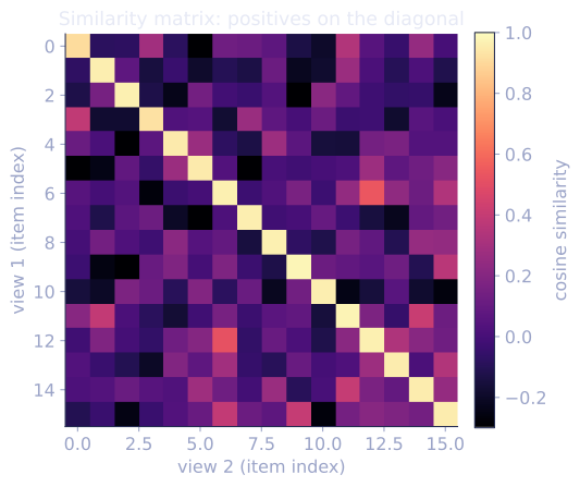
The aligned positives produce a low loss and high top-1 classification accuracy among the batch; shuffling breaks both.

Exercises

Exercise 1. A single anchor has one positive and $K$ negatives, all sharing the same similarity score $s$ with the anchor (the worst case for the model, positive indistinguishable from negatives). Show that the InfoNCE loss equals $\log(K + 1)$, independent of $\tau$, and explain why this is the random-guess floor.

Exercise 2. Take a perfectly aligned positive ($z^\top z^+ = 1$ for unit vectors) and a single negative at similarity $z^\top z^- = c$ with $-1 \le c < 1$. Write the loss as a function of $\tau$ and show it is increasing in $c$ and decreasing as $\tau \to 0$. What does the $\tau \to 0$ limit say about which negatives dominate the gradient?

Exercise 3 (code). Implement the cosine-similarity matrix and the symmetric InfoNCE loss directly in numpy. For a batch of $N$ unit embeddings where each anchor's positive is the row of a second matrix at the same index, verify that (a) when the two matrices are identical the loss is below its shuffled value, and (b) the per-row argmax recovers the diagonal as the predicted positive.

import numpy as np

rng = np.random.default_rng(0)
N, d = 32, 8

# View 1 and an aligned View 2 (small perturbation), both L2-normalized
z1 = rng.normal(size=(N, d))
z2 = z1 + 0.05 * rng.normal(size=(N, d))
z1 /= np.linalg.norm(z1, axis=1, keepdims=True)
z2 /= np.linalg.norm(z2, axis=1, keepdims=True)

def cosine_matrix(a, b):
    # rows already unit norm, so the dot product is cosine similarity
    return a @ b.T                                   # (N, N), S[i,j] = cos(a_i, b_j)

def info_nce(a, b, tau=0.1):
    s = cosine_matrix(a, b) / tau
    labels = np.arange(len(a))                       # positive of row i is column i
    # row-wise cross-entropy: -log softmax(s)[i, i]
    logsumexp = np.log(np.exp(s).sum(axis=1))
    row_loss = -(s[labels, labels] - logsumexp)
    return row_loss.mean()

def symmetric_info_nce(a, b, tau=0.1):
    return 0.5 * (info_nce(a, b, tau) + info_nce(b, a, tau))

loss_aligned = symmetric_info_nce(z1, z2)
perm = rng.permutation(N)
loss_shuffled = symmetric_info_nce(z1, z2[perm])

# (a) aligned loss is lower than shuffled
assert loss_aligned < loss_shuffled
# (b) argmax over each row recovers the diagonal positive
preds = cosine_matrix(z1, z2).argmax(axis=1)
assert np.array_equal(preds, np.arange(N))
print(round(loss_aligned, 4), round(loss_shuffled, 4))

The next lesson extends contrastive learning to cross-modal alignment with CLIP-style training, then surveys the non-contrastive alternatives.

References

- [1]Chen, T., Kornblith, S., Norouzi, M., & Hinton, G. (2020). "A simple framework for contrastive learning of visual representations (SimCLR)". ICML. arXiv:2002.05709. Augmented-view positives, large-batch negatives, and the projection head.↩
- [2]He, K., Fan, H., Wu, Y., Xie, S., & Girshick, R. (2020). "Momentum contrast for unsupervised visual representation learning (MoCo)". CVPR. arXiv:1911.05722. The momentum-encoder queue that decouples negatives from batch size.↩
- [3]Oord, A. van den, Li, Y., & Vinyals, O. (2018). "Representation learning with contrastive predictive coding (InfoNCE)". arXiv:1807.03748. Introduces the InfoNCE loss as a mutual-information lower bound.↩